Google Sheets Color Scale Formatting
Color Scale Formatting
Color Scales are premade types of conditional formatting in Google Sheets used to highlight cells in a range to indicate how large or small the cell values are.
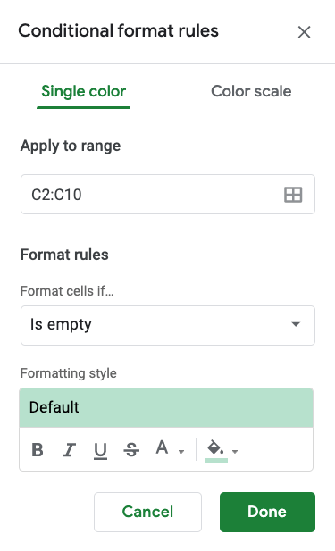
Here is the Color scale part of the conditional format rules menu:

You can access the menu by selecting the Conditional formatting option in the Format menu.
Color Scale Options
From the conditional format rules menu you can choose:
- Which cells the color scale applies to
- What colors the scale uses
- The min, mid, and max points
Apply to range
In the Apply to range field you can enter the cells and ranges that the color scale applies to.
You can enter cells and ranges separated by a comma , into the field.

You can also click the icon in the right of the field to select data ranges:
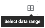
This will open a dialog box where you can add ranges by selection:

Custom color scale
You can customize the color scale by selecting min/mid/max point color icons on the right-hand side:
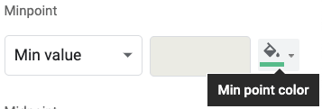
This will bring up a color picking menu. See the Format colors chapter for a detailed guide of how to customize colors.
Custom Min/Mid/Max Points
The color scale will apply relative to the chosen min/mid/max points.
The default option is Min/Max value:
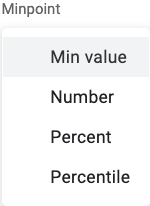
With the Min/Max value option, google sheets will choose the min and max points based on the largest and smallest values in the selected range.
The other options are:
- Number
- Percent
- Percentile
These options will let you specify precisely what the min, mid, and max points should be.
Color Scale Formatting Example (Min/Max Values)
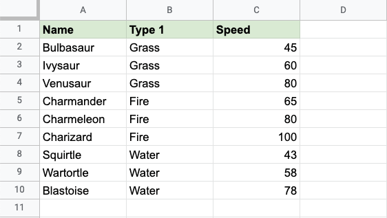
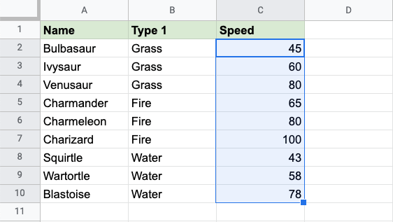
Highlight the Speed values of each Pokemon with Color scale conditional formatting.
Conditional formatting, step by step:
- Select the range of Speed values
C2:C10
- Click on the Conditional Formatting option in the Format menu

The Conditional Formatting menu will appear in the right-hand side of the spreadsheet:
- Select the Color Scales option

There are 9 default color scale options to choose from.
The color at the right-hand side of the icons ![]() will apply to the highest values by default.
will apply to the highest values by default.
- Click on the Preview scale "Choose Default Format"
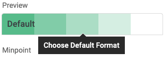
- Select the "White to green" Color scale

Now, the Speed value cells will have a colored background highlighting:
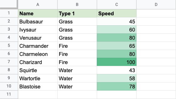
Dark green is used for the highest values, and white for the lowest values.
Charizard has the highest Speed value (100) and Squirtle has the lowest Speed value (43).
All the cells in the range gradually change color from dark green, to ligher greens and then to white.

