Google Sheets Single Color Formatting
Single Color Formatting
Single Color is a premade type of conditional formatting in Google Sheets used to apply a customizable formatting option to all the cells that match a condition.
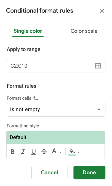
Here is the Single Color part of the conditional format rules menu:
You can access the menu by selecting the Conditional formatting option in the Format menu.
Single Color Options
From the conditional format rules menu you can choose:
- Which cells the conditional formatting applies to
- Which format rule is used
- The formatting style
Apply to range
In the Apply to range field you can enter the cells and ranges that the Single Color applies to.
You can enter cells and ranges separated by a comma , into the field.

You can also click the icon in the right of the field to select data ranges:

This will open a dialog box where you can add ranges by selection:

Format rules
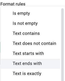
You can choose which rule to apply from the Format cells if... drop down menu. There are many options:
- Empty or not Empty cells
- Text Contains or not Contains
- Text Starts or Ends with
- Text is Exactly
- Calendar Dates
- Greater than
- Less than
- Equal to
- Between or not Between
- Custom rules
Formatting style
The Single Color formatting lets you customize both the background color and the font of the cells.

See the Format Colors chapter and Format Fonts chapter for detailed guides of how to customize colors and fonts.
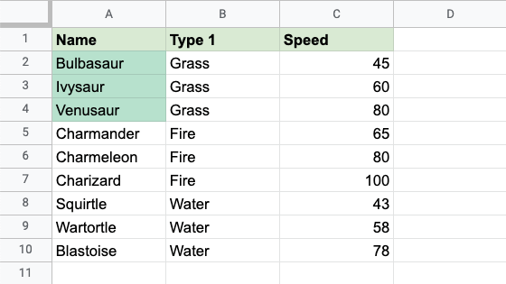
Single Color Formatting Example (Text Ends With)
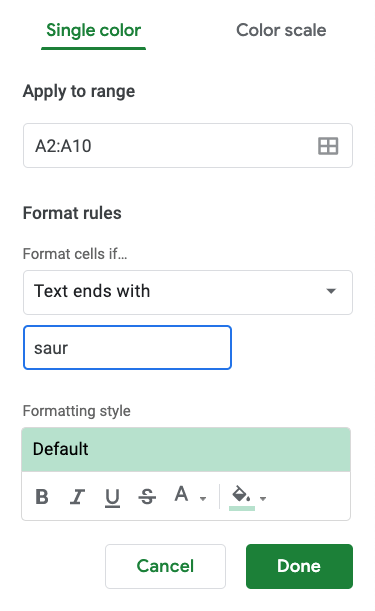
Highlight the Pokemon name values ending with saur with Single Color conditional formatting.
Conditional formatting, step by step:
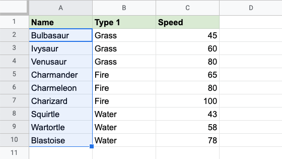
- Select the range of Name values
A2:A10
- Click on the Conditional Formatting option in the Format menu
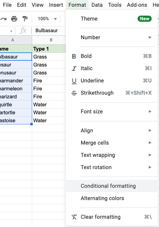
The Conditional Formatting menu will appear in the right-hand side of the spreadsheet:
- Select the Text ends with option from the Format rules drop-down menu:
- Type
saurin the input field:
Now, the Name value cells will have a colored background highlighting if the name ends with "saur":