Excel Top/Bottom Rules
Top/Bottom Rules
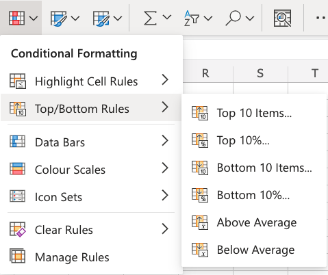
Top/Bottom Rules are premade types of conditional formatting in Excel used to change the appearance of cells in a range based on your specified conditions.
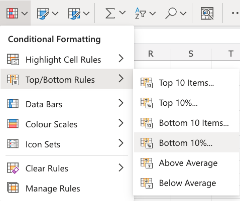
Here is the Top/Bottom Rules part of the conditional formatting menu:
Appearance Options
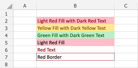
The web browser version of Excel offers the following appearance options for conditionally formatted cells:
- Light Red Fill with Dark Red Text
- Yellow Fill with Dark Yellow Text
- Green Fill with Dark Green Text
- Light Red Fill
- Red Text
- Red Border
Here is how the options look in a spreadsheet:
Top/Bottom 10 Items Example
The "Top 10 Items..." and "Bottom 10 Items..." rules will highlight cells with one of the appearance options based on the cell value being the top or bottom values in a range.
Note: The default number of items is 10, but you can specify any whole number up to 1000 for Top/Bottom Items to be highlighted.
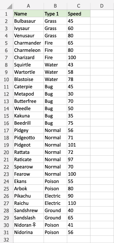
You can choose any range for where the Highlight Cell Rule should apply. It can be a few cells, a single column, a single row, or a combination of multiple cells, rows and columns.
Let's first apply the Top 10 Items... rule to the Speed values.
"Top 10 Items..." Rule, step by step:
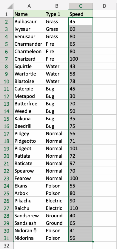
- Select the range
C2:C31for Speed values
- Click on the Conditional Formatting icon
 in the ribbon, from Home menu
 - Select Top/Bottom Rules from the drop-down menu
- Select Top 10 Items... from the menu

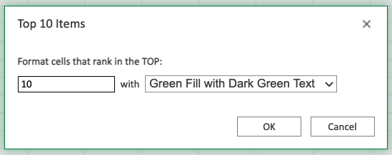
This will open a dialog box where you can specify the value and the appearance option.
- Leave the default value
10in the input field - Select the appearance option "Green Fill with Dark Green Text" from the dropdown menu
Now, the 10 cells with the top values will be highlighted in green:

Great! Now, the top 10 Speed values are easily identified.
Let's try the same with the bottom 10 Speed values.
Note: Multiple rules can be applied to the same range.
Repeat the steps, but instead choose Bottom 10 Items... in the menu and select the "Light Red Fill with Dark Red Text" appearance option.
Now, the slowest values are also highlighted:
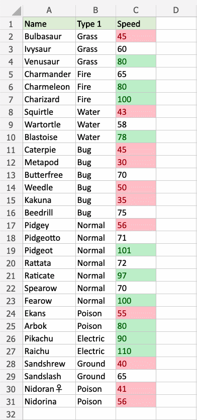
Notice that there are actually 11 items highlighted in red. Why could this be?
Let's sort the table with descending Speed values for a clue:
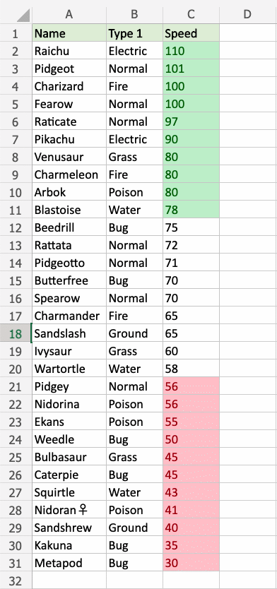
We can see that both Pidgey and Nidorina have a Speed of 56. So, they are tied for the 10th bottom value.
Note: When using the Top/Bottom 10... conditional formatting, values that tie will all be highlighted.
Top/Bottom 10% Example
The "Top 10%..." and "Bottom 10%..." rules will highlight cells with one of the appearance options based on the cell value being the top or bottom percent of values in a range.
Note: The default percent of items is 10, but you can specify any whole number up to 100 for Top/Bottom Percent to be highlighted.
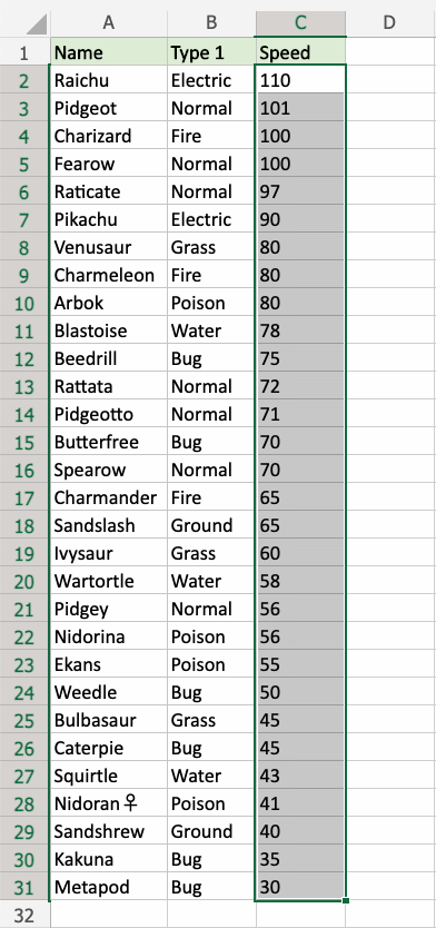
Let's apply Top and Bottom 10% rules to the same dataset with sorted Speed values:
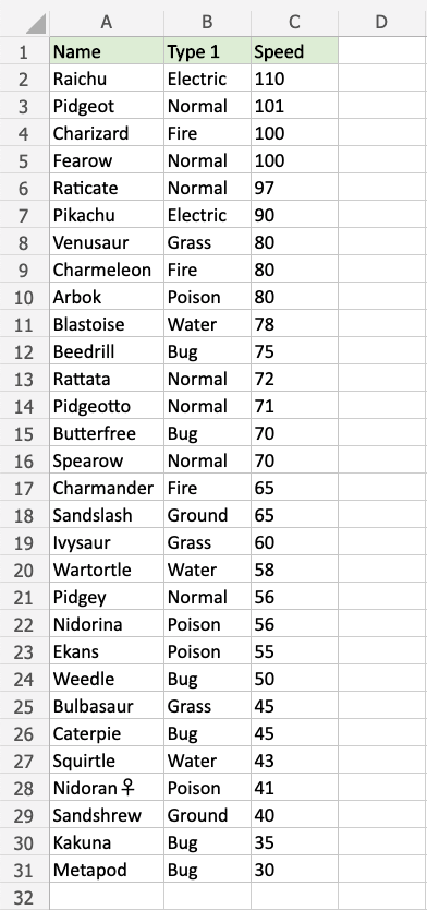
You can choose any range for where the Highlight Cell Rule should apply. It can be a few cells, a single column, a single row, or a combination of multiple cells, rows and columns.
Let's first apply the Bottom 10%... rule to the Speed values.
"Bottom 10%..." Rule, step by step:
- Select the range
C2:C31for Speed values
- Click on the Conditional Formatting icon in the ribbon, from Home menu
- Select Top/Bottom Rules from the drop-down menu
- Select Bottom 10%... from the menu
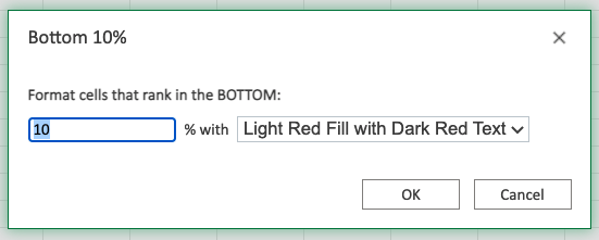
This will open a dialog box where you can specify the value and the appearance option.
- Leave the default value
10in the input field - Select the appearance option "Light Red Fill with Dark Red Text" from the dropdown menu
Now, the bottom 10% of cells will be highlighted in red:
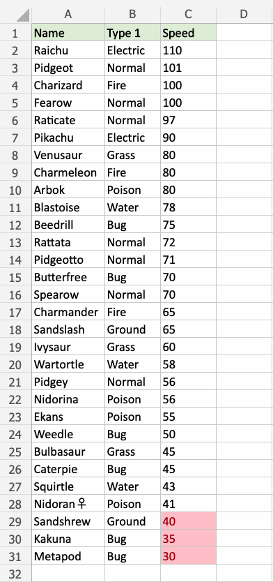
Notice that there are 3 highlighted cells.
There are 30 cells in the range, so 10% of that is 3 cells.
Note: The number of cells will be rounded down to the closest whole number based on the percent.
For example:
- 6% of 30 is 1.8, which will be rounded down to 1 cell
- 7% of 30 is 2.1, which will be rounded down to 2 cells
Let's try the same with the top 10% Speed values.
Repeat the steps, but instead choose Top 10%... in the menu and select the "Green Fill with Dark Green Text" appearance option.
Now, the fastest values are also highlighted:
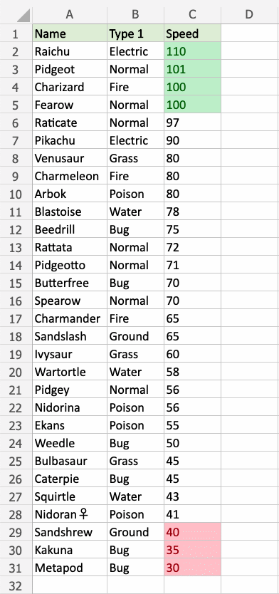
Notice that there are actually 4 items highlighted in green.
We can see that both Charizard and Fearow have a Speed of 100. So, they are tied for the 3rd top value.
Both are included in the top 10% and are highlighted.
Note: You can remove the Highlight Cell Rules with Manage Rules.

